AI Powered Drone Networks: Revolutionizing Early Crop Disease Detection in Smallholder Farms

The global agricultural sector faces an unprecedented challenge: feeding 9.7 billion people by 2050 while reducing environmental impact and supporting smallholder farmers who produce 70% of the world's food. Traditional crop disease management relies on visual inspection a method that detects problems only after significant damage has occurred. This article explores how AI-powered autonomous drone networks combined with multispectral imaging can detect crop diseases 7-14 days before visible symptoms appear, potentially saving 20-40% of annual crop losses and reducing pesticide use by 30-50%.

The Problem: Late Detection, High Losses

Current Challenges in Smallholder Agriculture

Smallholder farmers those cultivating less than 2 hectares face disproportionate challenges:

• Detection Delay: By the time diseases are visible to the naked eye, 15-30% of crop damage has already occurred
• Limited Expert Access: Agricultural extension workers serve 1,000+ farmers each, making timely field visits impossible
• Blanket Treatment: Without precise diagnosis, farmers apply pesticides preventively, increasing costs 40-60% and environmental contamination
• Economic Vulnerability: A single disease outbreak can devastate entire harvests; 30-50% of smallholder income goes to crop protection
• Climate Change Amplification: Warming temperatures expand disease vectors' geographic range by 2-3 latitude degrees per decade

The Scale of the Crisis

Global crop losses to diseases exceed $220 billion annually. In developing regions, post-harvest losses reach 30-40% compared to 5-10% in developed nations. For reference, wheat rust diseases alone cause $5 billion in annual losses globally, while late blight in potatoes accounts for $6 billion.

The Solution: Intelligent Aerial Surveillance

How Early Detection Changes Everything

Plant diseases trigger physiological changes before visible symptoms:

1. Cellular Disruption (Days 1-3): Pathogen infection alters leaf cell structure
2. Biochemical Changes (Days 3-7): Chlorophyll degradation begins, changing light reflectance patterns
3. Temperature Anomalies (Days 5-10): Stressed tissue shows 0.5-2°C temperature variations
4. Spectral Signature Shifts (Days 7-14): Changes in near-infrared (NIR) and red-edge reflectance
5. Visible Symptoms (Days 14-21): Lesions, wilting, discoloration appear to human eye

Critical Window: The 7-14 day pre-symptomatic period is when intervention is most effective and economic.

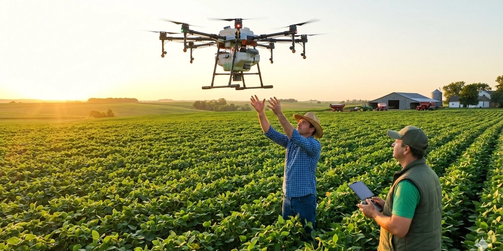
Why Drones and AI?

Drone Advantages:

• Coverage: A single drone can survey 50-100 hectares per flight (vs. 2-3 hectares/hour on foot)
• Frequency: Daily or weekly monitoring vs. monthly field visits
• Perspective: Overhead view reveals patterns invisible from ground level
• Access: Can survey difficult terrain, waterlogged fields, or dense canopy
• Data Quality: Consistent altitude and overlap ensure standardized imagery

AI Advantages:

• Speed: Analyzes thousands of images in minutes vs. days of manual inspection
• Precision: Detects subtle spectral changes invisible to human eyes
• Consistency: Eliminates human fatigue, bias, or variability
• Learning: Improves accuracy with every additional labeled dataset
• Scalability: Same model can serve thousands of farms simultaneously

System Architecture: From Flight to Recommendation

Hardware Components

1. Aerial Platform

• Multi-rotor UAV (quadcopter or hexacopter)
• Flight time: 25-35 minutes per battery
• Payload capacity: 500-1,000 grams
• Autonomous flight capability with waypoint navigation
• RTK-GPS for centimeter-level positioning accuracy

2. Imaging Sensors

Multispectral Camera:

• 5-10 spectral bands including:
  • Blue (450 nm): Chlorophyll absorption
  • Green (550 nm): Reflectance peak
  • Red (650 nm): Chlorophyll absorption
  • Red-Edge (730 nm): Vegetation transition zone
  • Near-Infrared (850 nm): Cellular structure
• Resolution: 2-5 megapixels per band
• Captures multiple bands simultaneously
• Global shutter for sharp images during motion

Thermal Camera (Optional):

• 640×512 pixel resolution
• Temperature range: -20°C to +150°C
• Detects water stress and inflammation

RGB Camera:

• 20+ megapixel high-resolution
• Provides visual reference and documentation
• Enables change detection over time

3. Ground Control Station

• Ruggedized tablet or laptop
• Mission planning software
• Real-time telemetry monitoring
• Weather station integration
• 4G/5G connectivity for data upload

4. Edge Processing Unit (Optional)

• NVIDIA Jetson or similar ARM-based GPU
• Enables on-drone preliminary analysis
• Reduces data transmission requirements
• Provides instant alerts for critical findings

Software Stack

Flight Management Layer

Mission Planning → Autonomous Navigation → Image Capture → Quality Control

Data Processing Pipeline

Raw Images → Calibration → Ortho-mosaic Generation → Vegetation Indices → Feature Extraction

Machine Learning Architecture

Stage 1: Image Pre-processing

• Radiometric calibration using reflectance panels
• Geometric correction and ortho-rectification
• Image stitching and mosaic generation
• Segmentation of vegetation vs. soil

Stage 2: Feature Engineering

Vegetation Indices (mathematical combinations revealing plant health):

• NDVI (Normalized Difference Vegetation Index) = (NIR – Red) / (NIR + Red)

  • Range: -1 to +1
  • Healthy crops: 0.6-0.9
  • Stressed crops: 0.2-0.5

• NDRE (Normalized Difference Red-Edge) = (NIR – RedEdge) / (NIR + RedEdge)

  • More sensitive to chlorophyll content than NDVI
  • Better for mid-late season crops

• GNDVI (Green NDVI) = (NIR – Green) / (NIR + Green)

  • Sensitive to chlorophyll concentration
  • Useful for assessing nitrogen status

• SAVI (Soil-Adjusted Vegetation Index) = ((NIR – Red) / (NIR + Red + L)) × (1 + L)

  • Minimizes soil brightness influence
  • Critical for early-season sparse canopy

Texture Features:

• GLCM (Gray-Level Co-occurrence Matrix) features: contrast, homogeneity, entropy
• Local Binary Patterns for leaf texture analysis
• Fourier descriptors for lesion shape characterization

Temporal Features:

• Rate of change in vegetation indices over 7-14 day windows
• Sudden drops indicating rapid disease progression
• Growth rate deviation from expected crop development curve

Stage 3: Machine Learning Models

Approach 1: Classical ML (Baseline)

• Random Forest or XGBoost classifier
• Input: 50-100 engineered features per image patch
• Output: Disease classification + confidence score
• Training: 10,000-50,000 labeled image patches
• Accuracy: 75-85% for well-differentiated diseases

Approach 2: Deep Learning (Advanced)

Convolutional Neural Network Architecture:

Input (5-10 channel multispectral image, 256x256 pixels)
    ↓
Conv Block 1: 32 filters, 3x3 kernel, ReLU, Batch Norm, MaxPool
    ↓
Conv Block 2: 64 filters, 3x3 kernel, ReLU, Batch Norm, MaxPool
    ↓
Conv Block 3: 128 filters, 3x3 kernel, ReLU, Batch Norm, MaxPool
    ↓
Conv Block 4: 256 filters, 3x3 kernel, ReLU, Batch Norm, MaxPool
    ↓
Global Average Pooling
    ↓
Dense Layer: 512 neurons, ReLU, Dropout (0.5)
    ↓
Output Layer: Softmax over disease classes + healthy + uncertain

Training Strategy:

• Transfer learning from ImageNet pre-trained models (ResNet50, EfficientNet)
• Fine-tuning on agricultural imagery
• Data augmentation: rotation, flip, brightness adjustment, spectral noise
• Class balancing through weighted loss function
• 5-fold cross-validation for robust evaluation

Accuracy Targets:

• Overall accuracy: 85-92%
• Per-disease precision: 80-95% (varies by disease distinctiveness)
• Early-stage detection: 70-85% (7-14 days pre-symptomatic)

Approach 3: Ensemble Methods

• Combine classical ML + deep learning predictions
• Weighted voting based on historical accuracy per disease
• Uncertainty quantification using ensemble disagreement
• Achieves 2-5% accuracy improvement over single models

Stage 4: Explainable AI Integration

Farmers and agronomists need to understand why the AI made its recommendation:

Techniques:

• Grad-CAM (Gradient-weighted Class Activation Mapping): Highlights image regions driving the prediction
• LIME (Local Interpretable Model-agnostic Explanations): Shows which features matter most
• Attention Maps: Visualizes what the model “looks at”
• Feature Importance Ranking: Lists top contributing factors

Output Example:

Disease: Late Blight (Phytophthora infestans)
Confidence: 87%
Affected Area: 12 square meters (2.3% of field)
Key Indicators:
  1. 35% drop in NDVI (weight: 0.42)
  2. 1.8°C temperature elevation (weight: 0.28)
  3. Water-soaked lesion texture (weight: 0.30)
Recommendation: Apply copper-based fungicide within 48 hours

Decision Support System

Recommendation Engine:

1. Disease identification + severity assessment
2. Treatment threshold calculation (economic injury level)
3. Product recommendation (pesticide/biocontrol/cultural practice)
4. Application timing and method
5. Cost-benefit analysis
6. Environmental impact assessment

Farmer Interface (Mobile App):

• Push notifications for detected issues
• Interactive map showing affected areas
• Photo documentation with time-series comparison
• Treatment instructions in local language
• Voice guidance for low-literacy users
• Direct connection to input suppliers
• Integration with local weather forecasts

Implementation Methodology

Phase 1: Baseline Data Collection

Objective: Build comprehensive disease database for local context

Activities:

1. Partner with agricultural research stations and universities
2. Collect samples of major crop diseases in your region
3. Conduct controlled infection experiments in greenhouse/field plots
4. Capture multispectral imagery at multiple disease stages
5. Record environmental conditions (temperature, humidity, rainfall)
6. Document disease progression timeline with daily imaging

Data Target: 5,000-10,000 images per major disease × 5-8 diseases = 25,000-80,000 training images

Key Considerations:

• Include healthy plants as negative class
• Capture multiple crop varieties (disease manifestation varies)
• Document co-occurring diseases (real-world complexity)
• Account for different growth stages
• Include various lighting conditions and viewing angles

Phase 2: Model Development and Validation

Training Pipeline:

# Pseudo-code for training workflow
for epoch in range(num_epochs):
    for batch in training_data:
        # Forward pass
        predictions = model(batch.images)
        loss = criterion(predictions, batch.labels)

        # Backward pass
        optimizer.zero_grad()
        loss.backward()
        optimizer.step()

    # Validation
    val_accuracy = evaluate(model, validation_data)

    # Early stopping check
    if val_accuracy > best_accuracy:
        save_model(model)
        best_accuracy = val_accuracy

Validation Strategy:

• Split data: 70% training, 15% validation, 15% testing
• Temporal validation: train on earlier data, test on recent data
• Spatial validation: train on some farms, test on different farms
• Cross-crop validation: test model generalization across varieties

Performance Metrics:

• Accuracy, Precision, Recall, F1-Score per disease class
• Confusion matrix to identify misclassification patterns
• ROC curves and AUC for threshold optimization
• Detection timing: days before visible symptoms
• Inference speed: images processed per second

Phase 3: Pilot Deployment

Farm Selection Criteria:

• 10-15 farms representing diverse conditions
• Mix of crop types (wheat, rice, maize, vegetables)
• Range of farm sizes (0.5-5 hectares)
• Varying disease pressure histories
• Farmers willing to follow recommendations and document results

Flight Protocol:

• Weekly flights during critical growth periods
• Consistent flight parameters: 30m altitude, 75% image overlap
• Morning flights (8-11 AM) for optimal lighting and minimal wind
• Pre-flight calibration using reflectance panels
• Post-flight data quality check before leaving site

Monitoring and Feedback:

• Weekly farmer interviews about detected issues
• Ground-truthing: physical scouting of flagged areas
• Documentation of treatments applied and outcomes
• Collection of misclassification examples for model refinement
• Iterative model updates every 2-4 weeks

Phase 4: Impact Assessment

Economic Metrics:

• Yield comparison: pilot farms vs. control farms
• Pesticide cost reduction ($/hectare)
• Treatment timing improvement (days gained)
• Labor savings (hours per hectare)
• Return on investment (benefit/cost ratio)

Environmental Metrics:

• Pesticide volume reduction (liters/hectare)
• Active ingredient reduction (kg/hectare)
• Targeted vs. blanket application ratio
• Pesticide drift reduction
• Beneficial insect population surveys
• Soil and water quality testing

Agronomic Metrics:

• Disease incidence reduction (% infected plants)
• Disease severity reduction (scale 0-10)
• Yield increase (kg/hectare)
• Crop quality improvement (grade distribution)

Social Metrics:

• Farmer satisfaction surveys (1-5 Likert scale)
• Technology adoption rate
• Knowledge transfer effectiveness
• Farmer confidence in decision-making
• Reduction in anxiety about crop health

Target Outcomes:

• 20-30% yield increase through early intervention
• 25-35% reduction in pesticide costs
• 40-50% reduction in unnecessary treatments
• 85%+ farmer satisfaction rate
• Economic payback period: 2-3 growing seasons

Technical Challenges and Solutions

Challenge 1: Spectral Variability

Problem: Multispectral reflectance varies with sun angle, cloud cover, sensor calibration drift

Solution:

• Empirical line calibration using ground reference panels before/after each flight
• Bidirectional Reflectance Distribution Function (BRDF) correction
• Cloud shadow detection and removal algorithms
• Atmospheric correction models (e.g., 6S radiative transfer)
• Time-of-day normalization using solar zenith angle

Challenge 2: Class Imbalance

Problem: Healthy crops vastly outnumber diseased patches (ratio 100:1 or higher)

Solution:

• Focal loss function emphasizing rare classes
• Synthetic minority oversampling (SMOTE adapted for images)
• Hard negative mining: focus training on misclassified examples
• Two-stage detection: general health screening → detailed disease classification
• Anomaly detection approach for rare diseases

Challenge 3: Mixed Infections and Abiotic Stress

Problem: Multiple diseases co-occur; nutrient deficiency mimics disease symptoms

Solution:

• Multi-label classification allowing multiple simultaneous diagnoses
• Feature importance analysis to differentiate biotic vs. abiotic stress
• Temporal analysis: diseases progress differently than deficiencies
• Integration with soil testing data and farm management history
• Agronomist validation for ambiguous cases

Challenge 4: Phenological Variation

Problem: Crop appearance changes dramatically with growth stage; same disease looks different in seedling vs. mature plant

Solution:

• Growth stage classification as first step
• Stage-specific disease models
• Normalized features accounting for expected crop development
• Longitudinal modeling: track individual plants over time
• Include crop calendar and planting date in model inputs

Challenge 5: Computational Constraints

Problem: Rural areas lack reliable internet; edge devices have limited processing power

Solution:

• Model compression: pruning, quantization (FP32 → INT8)
• Knowledge distillation: train compact “student” model from large “teacher” model
• Progressive inference: quick screening → detailed analysis only for anomalies
• Offline operation mode with batch uploads when connectivity available
• Edge-cloud hybrid: lightweight detection on-drone, full analysis in cloud

Economic Model: Making it Sustainable

Cost Structure (Per Farm Service Model)

Capital Expenditure (One-time):

• Drone platform: $2,000-5,000
• Multispectral camera: $3,000-8,000
• Thermal camera (optional): $2,000-5,000
• Ground control station: $1,000-2,000
• Processing computer: $1,500-3,000
• Software licenses: $500-2,000
• Training and certification: $500-1,000
  Total: $10,500-26,000

Operational Expenditure (Annual per 100 farms):

• Batteries and maintenance: $1,000-2,000
• Insurance: $500-1,500
• Data storage and computing: $1,000-3,000
• Personnel (pilot/analyst part-time): $8,000-15,000
• Transport and logistics: $1,000-2,000
  Total: $11,500-23,500

Revenue Models

Model 1: Subscription Service

• $50-150 per hectare per season
• Includes 8-12 flights during critical periods
• Disease alerts and treatment recommendations
• For 100 farms × 2 hectares average × $100/ha = $20,000/season
• 2 seasons/year = $40,000 annual revenue

Model 2: Pay-Per-Flight

• $15-30 per hectare per flight
• Flexibility for farmers to choose frequency
• Lower commitment barrier

Model 3: Cooperative Ownership

• 20-50 farmers co-invest in drone + operator
• Share equipment costs and operational expenses
• Builds community capacity and ownership

Model 4: Government/NGO Subsidy

• Free or heavily subsidized service to smallholders
• Funded through agricultural development programs
• Demonstrated ROI justifies public investment

Break-Even Analysis

Conservative Scenario (100 farms, $100/ha/season, 2 seasons):

• Annual Revenue: $40,000
• Annual Costs: $23,500 (operations) + $5,000 (depreciation)
• Annual Profit: $11,500
• Payback Period: 18-24 months

Scaling Economics:

• At 200 farms: $80,000 revenue, $30,000 costs → $50,000 profit
• At 500 farms: $200,000 revenue, $50,000 costs → $150,000 profit
• Fixed costs plateau; marginal cost per farm drops significantly

Environmental and Social Impact

Environmental Benefits

Pesticide Reduction:

• Targeted application reduces total pesticide volume by 30-50%
• Early detection enables softer, less toxic interventions
• Prevents secondary pest problems from broad-spectrum chemicals
• Reduces pesticide residues on food by 40-60%

Water Quality Protection:

• Less chemical runoff into streams and groundwater
• Preservation of aquatic ecosystems
• Reduced human exposure through drinking water

Biodiversity Conservation:

• Beneficial insect populations recover (bees, ladybugs, predatory wasps)
• Bird populations increase with more invertebrate food sources
• Soil microbiome diversity improves with reduced chemical stress

Climate Mitigation:

• Increased yields reduce pressure for agricultural expansion (forest clearing)
• Reduced pesticide production energy footprint
• Healthier soils sequester more carbon

Quantified Impact (per 100 hectares):

• 500-1,500 kg less pesticide active ingredient annually
• 5-15 tons CO₂-equivalent reduction
• 50-100 bird species richness increase
• 20-40% increase in pollinator abundance

Social Benefits

Economic Empowerment:

• 20-30% income increase for participating farmers
• Reduced catastrophic crop loss risk
• Increased creditworthiness and access to loans
• Women farmers gain technical empowerment

Health Improvements:

• Reduced pesticide exposure for farm workers (50-70% less handling)
• Fewer acute poisoning incidents (10,000+ annually in developing countries)
• Long-term chronic disease risk reduction
• Improved safety for children in farming households

Knowledge Transfer:

• Farmers develop digital literacy and data interpretation skills
• Understanding of plant pathology fundamentals
• Strengthened farmer-agronomist relationships
• Youth engagement in agriculture through technology

Food Security:

• 10-20% increase in local food availability
• Price stabilization through reduced supply shocks
• Improved nutrition from reduced pesticide residues

Scaling Strategy

Phase 1: Proof of Concept (Year 1)

• 10-15 farms, single region
• Validate technical feasibility
• Establish baseline metrics
• Build farmer trust

Phase 2: Regional Expansion (Years 2-3)

• 100-200 farms across 3-5 districts
• Diversify crop types and agroecological zones
• Train local operators and agronomists
• Establish regional hubs

Phase 3: National Network (Years 4-5)

• 1,000-2,000 farms nationwide
• Franchise or cooperative model
• Government partnership and policy integration
• National disease surveillance network

Phase 4: Cross-Border Replication (Years 6+)

• Adapt to neighboring countries
• Open-source model and datasets
• International research collaborations
• South-South knowledge exchange

Future Enhancements

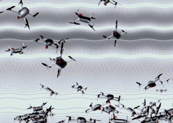
Autonomous Swarm Operations

• Multiple drones coordinate to survey large areas simultaneously
• Real-time communication and task allocation
• 5-10x coverage improvement

Predictive Modeling

• Weather-disease forecasting models
• Regional outbreak prediction 7-14 days ahead
• Preventive treatment recommendations
• Seasonal planning optimization

Integrated Pest Management

• Insect pest detection (not just diseases)
• Weed identification and mapping
• Beneficial organism monitoring
• Holistic farm health dashboard

Blockchain Integration

• Immutable spray records for food safety certification
• Traceability from farm to consumer
• Premium pricing for sustainably produced crops

AI-Powered Agronomic Advisory

• Personalized crop management recommendations
• Fertilization optimization
• Irrigation scheduling
• Harvest timing prediction

Conclusion

AI-powered drone networks represent a paradigm shift in agricultural disease management from reactive crisis response to proactive prevention. For smallholder farmers, this technology democratizes access to precision agriculture tools previously available only to large commercial operations.

The convergence of affordable drones, powerful edge computing, advanced machine learning, and mobile connectivity creates an unprecedented opportunity to transform the lives of millions of farmers while simultaneously addressing environmental sustainability challenges.

This is not science fiction the technology exists today. What's needed is integration, validation, and deployment at scale. With the right technical skills, agronomic knowledge, and commitment to smallholder welfare, we can build systems that feed the world sustainably.

The question is not whether this transformation will happen, but how quickly and whether smallholder farmers will be included in this agricultural revolution or left behind.