Understanding RL Vision

Our CoinRun model

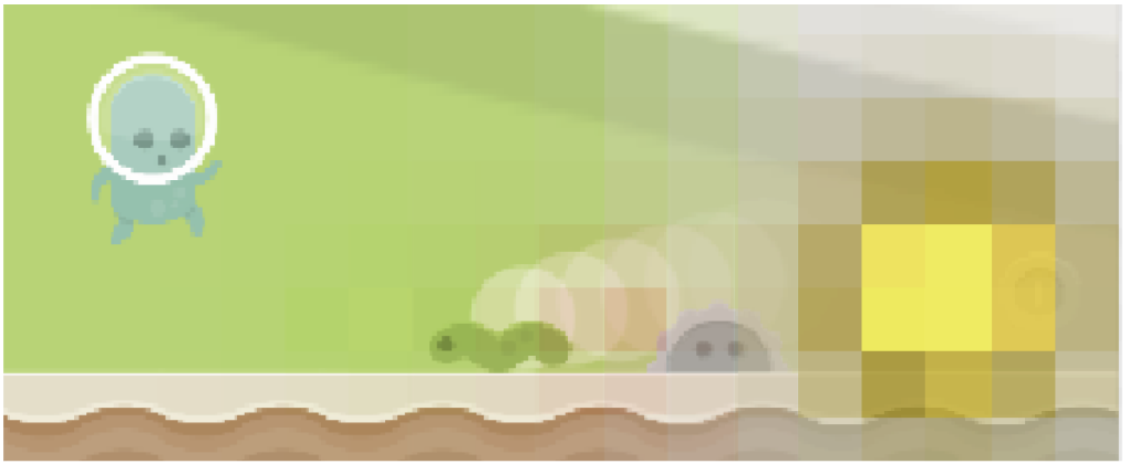
CoinRun is a side-scrolling platformer in which the agent must dodge enemies and other traps and collect the coin at the end of the level.

CoinRun is procedurally-generated, meaning that each new level encountered by the agent is randomly generated from scratch. This incentivizes the model to learn how to spot the different kinds of objects in the game, since it cannot get away with simply memorizing a small number of specific trajectories .We use the original version of CoinRun , not the version from Procgen Benchmark , which is slightly different. To play CoinRun yourself, please follow the instructions here.

Here are some examples of the objects used, along with walls and floors, to generate CoinRun levels.

There are 9 actions available to the agent in CoinRun:

We trained a convolutional neural network on CoinRun for around 2 billion timesteps, using PPO , an actor-critic algorithm.We used the standard PPO hyperparameters for CoinRun , except that we used twice as many copies of the environment per worker and twice and many workers. The effect of these changes was to increase the effective batch size, which seemed to be necessary to reach the same performance with our smaller architecture. The architecture of our network is described in Appendix C. We used a non-recurrent network, to avoid any need to visualize multiple frames at once. Thus our model observes a single downsampled 64×64 image, and outputs a value function (an estimate of the total future time-discounted reward) and a policy (a probability distribution over the actions, from which the next action is sampled).

Since the only available reward is a fixed bonus for collecting the coin, the value function estimates the time-discountedWe use a discount rate of 0.999 per timestep. probability that the agent will successfully complete the level.

Model analysis

Having trained a strong RL agent, we were curious to see what it had learned. Following , we developed an interface for examining trajectories of the agent playing the game. This incorporates attribution from a hidden layer that recognizes objects, which serves to highlight objects that positively or negatively influence a particular network output. By applying dimensionality reduction, we obtain attribution vectors whose components correspond to different types of object, which we indicate using different colors.

Here is our interface for a typical trajectory, with the value function as the network output. It reveals the model using obstacles, coins, enemies and more to compute the value function.

Dissecting failure

Our fully-trained model fails to complete around 1 in every 200 levels. We explored a few of these failures using our interface, and found that we were usually able to understand why they occurred.

The failure often boils down to the fact that the model has no memory, and must therefore choose its action based only on the current observation. It is also common for some unlucky sampling of actions from the agent’s policy to be partly responsible.

Here are some cherry-picked examples of failures, carefully analyzed step-by-step.

Hallucinations

We searched for errors in the model using generalized advantage estimation (GAE) ,We use the same GAE hyperparameters as in training, namely $\gamma=0.999$ and $\lambda=0.95$. which measures how successful each action turned out relative to the agent’s expectations. An unusually high or low GAE indicates that either something unexpected occurred, or the agent’s expectations were miscalibrated. Filtering for such timesteps can therefore find problems with the value function or policy.

Using our interface, we found a couple of cases in which the model “hallucinated” a feature not present in the observation, causing the value function to spike.

Model editing

Our analysis so far has been mostly qualitative. To quantitatively validate our analysis, we hand-edited the model to make the agent blind to certain features identified by our interface: buzzsaw obstacles in one case, and left-moving enemies in another. Our method for this can be thought of as a primitive form of circuit-editing , and we explain it in detail in Appendix A.

We evaluated each edit by measuring the percentage of levels that the new agent failed to complete, broken down by the object that the agent collided with to cause the failure. Our results show that our edits were successful and targeted, with no statistically measurable effects on the agent’s other abilities.The data for this plot are as follows.
Percentage of levels failed due to: buzzsaw obstacle / enemy moving left / enemy moving right / multiple or other:
– Original model: 0.37% / 0.16% / 0.12% / 0.08%
– Buzzsaw obstacle blindness: 12.76% / 0.16% / 0.08% / 0.05%
– Enemy moving left blindness: 0.36% / 4.69% / 0.97% / 0.07%
Each model was tested on 10,000 levels.

We did not manage to achieve complete blindness, however: the buzzsaw-edited model still performed significantly better than the original model did when we made the buzzsaws completely invisible.Our results on the version of the game with invisible buzzsaws are as follows.
Percentage of levels failed due to: buzzsaw obstacle / enemy moving left / enemy moving right / multiple or other:
Original model, invisible buzzsaws: 32.20% / 0.05% / 0.05% / 0.05%
We tested the model on 10,000 levels.
We experimented briefly with iterating the editing procedure, but were not able to achieve more than around 50% buzzsaw blindness by this metric without affecting the model’s other abilities. This implies that the model has other ways of detecting buzzsaws than the feature identified by our interface.

Here are the original and edited models playing some cherry-picked levels.

The diversity hypothesis

All of the above analysis uses the same hidden layer of our network, the third of five convolutional layers, since it was much harder to find interpretable features at other layers. Interestingly, the level of abstraction at which this layer operates – finding the locations of various in-game objects – is exactly the level at which CoinRun levels are randomized using procedural generation. Furthermore, we found that training on many randomized levels was essential for us to be able to find any interpretable features at all.

This led us to suspect that the diversity introduced by CoinRun’s randomization is linked to the formation of interpretable features. We call this the diversity hypothesis:

Interpretable features tend to arise (at a given level of abstraction) if and only if the training distribution is diverse enough (at that level of abstraction).

Our explanation for this hypothesis is as follows. For the forward implication (“only if”), we only expect features to be interpretable if they are general enough, and when the training distribution is not diverse enough, models have no incentive to develop features that generalize instead of overfitting. For the reverse implication (“if”), we do not expect it to hold in a strict sense: diversity on its own is not enough to guarantee the development of interpretable features, since they must also be relevant to the task. Rather, our intention with the reverse implication is to hypothesize that it holds very often in practice, as a result of generalization being bottlenecked by diversity.

In CoinRun, procedural generation is used to incentivize the model to learn skills that generalize to unseen levels . However, only the layout of each level is randomized, and correspondingly, we were only able to find interpretable features at the level of abstraction of objects. At a lower level, there are only a handful of visual patterns in the game, and the low-level features of our model seem to consist mostly of memorized color configurations used for picking these out. Similarly, the game’s high-level dynamics follow a few simple rules, and accordingly the high-level features of our model seem to involve mixtures of combinations of objects that are hard to decipher. To explore the other convolutional layers, see the interface here.

Interpretability and generalization

To test our hypothesis, we made the training distribution less diverse, by training the agent on a fixed set of 100 levels. This dramatically reduced our ability to interpret the model’s features. Here we display an interface for the new model, generated in the same way as the one above. The smoothly increasing value function suggests that the model has memorized the number of timesteps until the end of the level, and the features it uses for this focus on irrelevant background objects. Similar overfitting occurs for other video games with a limited number of levels .

We attempted to quantify this effect by varying the number of levels used to train the agent, and evaluating the 8 features identified by our interface on how interpretable they were.The interfaces used for this evaluation can be found here. Features were scored based on how consistently they focused on the same objects, and whether the value function attribution made sense – for example, background objects should not be relevant. This process was subjective and noisy, but that may be unavoidable. We also measured the generalization ability of each model, by testing the agent on unseen levels .The data for this plot are as follows.
– Number of training levels: 100 / 300 / 1000 / 3,000 / 10,000 / 30,000 / 100,000
– Percentage of levels completed (train, run 1): 99.96% / 99.82% / 99.67% / 99.65% / 99.47% / 99.55% / 99.57%
– Percentage of levels completed (train, run 2): 99.97% / 99.86% / 99.70% / 99.46% / 99.39% / 99.50% / 99.37%
– Percentage of levels completed (test, run 1): 61.81% / 66.95% / 74.93% / 89.87% / 97.53% / 98.66% / 99.25%
– Percentage of levels completed (test, run 2): 64.13% / 67.64% / 73.46% / 90.36% / 97.44% / 98.89% / 99.35%
– Percentage of features interpretable (researcher 1, run 1): 52.5% / 22.5% / 11.25% / 45% / 90% / 75% / 91.25%
– Percentage of features interpretable (researcher 2, run 1): 8.75% / 8.75% / 10% / 26.25% / 56.25% / 90% / 70%
– Percentage of features interpretable (researcher 1, run 2): 15% / 13.75% / 15% / 23.75% / 53.75% / 90% / 96.25%
– Percentage of features interpretable (researcher 2, run 2): 3.75% / 6.25% / 21.25% / 45% / 72.5% / 83.75% / 77.5%
Percentages of levels completed are estimated by sampling 10,000 levels with replacement.

Our results illustrate how diversity may lead to interpretable features via generalization, lending support to the diversity hypothesis. Nevertheless, we still consider the hypothesis to be highly unproven.

Feature visualization

Feature visualization answers questions about what certain parts of a network are looking for by generating examples. This can be done by applying gradient descent to the input image, starting from random noise, with the objective of activating a particular neuron or group of neurons. While this method works well for an image classifier trained on ImageNet , for our CoinRun model it yields only featureless clouds of color. Only for the first layer, which computes simple convolutions of the input, does the method produce comparable visualizations for the two models.

Gradient-based feature visualization has previously been shown to struggle with RL models trained on Atari games . To try to get it to work for CoinRun, we varied the method in a number of ways. Nothing we tried had any noticeable effect on the quality of the visualizations.

• Transformation robustness. This is the method of stochastically jittering, rotating and scaling the image between optimization steps, to search for examples that are robust to these transformations . We tried both increasing and decreasing the size of the jittering. Rotating and scaling are less appropriate for CoinRun, since the observations themselves are not invariant to these transformations.
• Penalizing extremal colors.By an “extremal” color we mean one of the 8 colors with maximal or minimal RGB values (black, white, red, green, blue, yellow, cyan and magenta). Noticing that our visualizations tend to use extremal colors towards the middle, we tried including in the visualization objective an L2 penalty of various strengths on the activations of the first layer, which successfully reduced the size of the extremally-colored region but did not otherwise help.
• Alternative objectives. We tried using an alternative optimization objective , such as the caricature objective.The caricature objective is to maximize the dot product between the activations of the input image and the activations of a reference image. Caricatures are often an especially easy type of feature visualization to make work, and helpful for getting a first glance into what features a model has. They are demonstrated in this notebook. A more detailed manuscript by its authors is forthcoming. We also tried using dimensionality reduction, as described below, to choose non-axis-aligned directions in activation space to maximize.
• Low-level visual diversity. In an attempt to broaden the distribution of images seen by the model, we retrained it on a version of the game with procedurally-generated sprites. We additionally tried adding noise to the images, both independent per-pixel noise and spatially-correlated noise. Finally, we experimented briefly with adversarial training , though we did not pursue this line of inquiry very far.

As shown below, we were able to use dataset examples to identify a number of channels that pick out human-interpretable features. It is therefore striking how resistant gradient-based methods were to our efforts. We believe that this is because solving CoinRun does not ultimately require much visual ability. Even with our modifications, it is possible to solve the game using simple visual shortcuts, such as picking out certain small configurations of pixels. These shortcuts work well on the narrow distribution of images on which the model is trained, but behave unpredictably in the full space of images in which gradient-based optimization takes place.

Our analysis here provides further insight into the diversity hypothesis. In support of the hypothesis, we have examples of features that are hard to interpret in the absence of diversity. But there is also evidence that the hypothesis may need to be refined. Firstly, it seems to be a lack of diversity at a low level of abstraction that harms our ability to interpret features at all levels of abstraction, which could be due to the fact that gradient-based feature visualization needs to back-propagate through earlier layers. Secondly, the failure of our efforts to increase low-level visual diversity suggests that diversity may need to be assessed in the context of the requirements of the task.

Dataset example-based feature visualization

As an alternative to gradient-based feature visualization, we use dataset examples. This idea has a long history, and can be thought of as a heavily-regularized form of feature visualization . In more detail, we sample a few thousand observations infrequently from the agent playing the game, and pass them through the model. We then apply a dimensionality reduction method known as non-negative matrix factorization (NMF) to the activation channels .More precisely, we find a non-negative approximate low-rank factorization of the matrix obtained by flattening the spatial dimensions of the activations into the batch dimension. This matrix has one row per observation per spatial position and one column per channel: thus the dimensionality reduction does not use spatial information. For each of the resulting channels (which correspond to weighted combinations of the original channels), we choose the observations and spatial positions with the strongest activation (with a limited number of examples per position, for diversity), and display a patch from the observation at that position.

Unlike gradient-based feature visualization, this method finds some meaning to the different directions in activation space. However, it may still fail to provide a complete picture for each direction, since it only shows a limited number of dataset examples, and with limited context.

Spatially-aware feature visualization

CoinRun observations differ from natural images in that they are much less spatially invariant. For example, the agent always appears in the center, and the agent’s velocity is always encoded in the top left. As a result, some features detect unrelated things at different spatial positions, such as reading the agent’s velocity in the top left while detecting an unrelated object elsewhere. To account for this, we developed a spatially-aware version of dataset example-based feature visualization, in which we fix each spatial position in turn, and choose the observation with the strongest activation at that position (with a limited number of reuses of the same observation, for diversity). This creates a spatial correspondence between visualizations and observations.

Here is such a visualization for a feature that responds strongly to coins. The white squares in the top left show that the feature also responds strongly to the horizontal velocity info when it is white, corresponding to the agent moving right at full speed.

Attribution

Attribution answers questions about the relationships between neurons. It is most commonly used to see how the input to a network affects a particular output – for example, in RL – but it can also be applied to the activations of hidden layers . Although there are many approaches to attribution we could have used, we chose the method of integrated gradients . We explain in Appendix B how we applied this method a hidden layer, and how positive value function attribution can be thought of as “good news” and negative value function attribution can as “bad news”.

Dimensionality reduction for attribution

We showed above that a dimensionality reduction method known as non-negative matrix factorization (NMF) could be applied to the channels of activations to produce meaningful directions in activation space . We found that it is even more effective to apply NMF not to activations, but to value function attributionsAs before, we obtain the NMF directions by sampling a few thousand observations infrequently from the agent playing the game, computing the attributions, flattening the spatial dimensions into the batch dimension, and applying NMF. (working around the fact that NMF can only be applied to non-negative matricesOur workaround is to separate out the positive and negative parts of the attributions and concatenate them along the batch dimension. We could also have concatenated them along the channel dimension.). Both methods tend to produce NMF directions that are close to one-hot, and so can be thought of as picking out the most relevant channels. However, when reducing to a small number of dimensions, using attributions usually picks out more salient features, because attribution takes into account not just what neurons respond to but also whether their response matters.

Following , after applying NMF to attributions, we visualize them by assigning a different color to each of the resulting channels. We overlay these visualizations over the observation and contextualize each channel using feature visualization , making use of dataset example-based feature visualization. This gives a basic version of our interface, which allows us to see the effect of the main features at different spatial positions.

For the full version of our interface, we simply repeat this for an entire trajectory of the agent playing the game. We also incorporate video controls, a timeline view of compressed observations , and additional information, such as model outputs and sampled actions. Together these allow the trajectory to be easily explored and understood.

Attribution discussion

Attributions for our CoinRun model have some interesting properties that would be unusual for an ImageNet model.

• Sparsity. Attribution tends to be concentrated in a very small number of spatial positions and (post-NMF) channels. For example, in the figure above, the top 10 position–channel pairs account for more than 80% of the total absolute attribution. This might be explained by our earlier hypothesis that the model identifies objects by picking out certain small configurations of pixels. Because of this sparsity, we smooth out attribution over nearby spatial positions for the full version of our interface, so that the amount of visual space taken up can be used to judge attribution strength. This trades off some spatial precision for more precision with magnitudes.
• Unexpected sign. Value function attribution usually has the sign one would expect: positive for coins, negative for enemies, and so on. However, this is sometimes not the case. For example, in the figure above, the red channel that detects buzzsaw obstacles has both positive and negative attribution in two neighboring spatial positions towards the left. Our best guess is that this phenomenon is a result of statistical collinearity, caused by certain correlations in the procedural level generation together with the agent’s behavior. These could be visual, such as correlations between nearby pixels, or more abstract, such as both coins and long walls appearing at the end of every level. As a toy example, supposing the value function ought to increase by 2% when the end of the level becomes visible, the model could either increase the value function by 1% for coins and 1% for long walls, or by 3% for coins and −1% for long walls, and the effect would be similar.
• Outlier frames. When an unusual event causes the network to output extreme values, attribution can behave especially strangely. For example, in the buzzsaw hallucination frame, most features have a significant amount of both positive and negative attribution. We do not have a good explanation for this, but perhaps features are interacting in more complicated ways than usual. Moreover, in these cases there is often a significant component of the attribution lying outside the space spanned by the NMF directions, which we display as an additional “residual” feature. This could be because each frame is weighted equally when computing NMF, so outlier frames have little influence over the NMF directions.

These considerations suggest that some care may be required when interpreting attributions.

Questions for further research

The diversity hypothesis

1. Validity. Does the diversity hypothesis hold in other contexts, both within and outside of reinforcement learning?
2. Relationship to generalization. What is the three-way relationship between diversity, interpretable features and generalization? Do non-interpretable features indicate that a model will fail to generalize in certain ways? Generalization refers implicitly to an underlying distribution – how should this distribution be chosen?For example, to measure generalization for CoinRun models trained on a limited number of levels, we used the distribution over all possible procedurally-generated levels. However, to formalize the sense in which CoinRun is not diverse in its visual patterns or dynamics rules, one would need a distribution over levels from a wider class of games.
3. Caveats. How are interpretable features affected by other factors, such as the choice of task or algorithm, and how do these interact with diversity? Speculatively, do big enough models obtain interpretable features via the double descent phenomenon , even in the absence of diversity?
4. Quantification. Can we quantitatively predict how much diversity is needed for interpretable features, perhaps using generalization metrics? Can we be precise about what is meant by an “interpretable feature” and a “level of abstraction”?

Interpretability in the absence of diversity

1. Pervasiveness of non-diverse features. Do “non-diverse features”, by which we mean the hard-to-interpret features that tend to arise in the absence of diversity, remain when diversity is present? Is there a connection between these non-diverse features and the “non-robust features” that have been posited to explain adversarial examples ?
2. Coping with non-diverse levels of abstraction. Are there levels of abstraction at which even broad distributions like ImageNet remain non-diverse, and how can we best interpret models at these levels of abstraction?
3. Gradient-based feature visualization. Why does gradient-based feature visualization break down in the absence of diversity, and can it be made to work using transformation robustness, regularization, data augmentation, adversarial training, or other techniques? What property of the optimization leads to the clouds of extremal colors?
4. Trustworthiness of dataset examples and attribution. How reliable and trustworthy can we make very heavily-regularized versions of feature visualization, such as those based on dataset examples?Heavily-regularized feature visualization may be untrustworthy by failing to separate the things causing certain behavior from the things that merely correlate with those causes . What explains the strange behavior of attribution, and how trustworthy is it?

Interpretability in the RL framework

1. Non-visual and abstract features. What are the best methods for interpreting models with non-visual inputs? Even vision models may also have interpretable abstract features, such as relationships between objects or anticipated events: will any method of generating examples be enough to understand these, or do we need an entirely new approach? For models with memory, how can we interpret their hidden states ?
2. Improving reliability. How can we best identify, understand and correct rare failures and other errors in RL models? Can we actually improve models by model editing, rather than merely degrading them?
3. Modifying training. In what ways can we train RL models to make them more interpretable without a significant performance cost, such as by altering architectures or adding auxiliary predictive losses?
4. Leveraging the environment. How can we enrich interfaces using RL-specific data, such as trajectories of agent–environment interaction, state distributions, and advantage estimates? What are the benefits of incorporating user–environment interaction, such as for exploring counterfactuals?

What we would like to see from further research and why

We are motivated to study interpretability for RL for two reasons.

• To be able to interpret RL models. RL can be applied to an enormous variety of tasks, and seems likely to be a part of increasingly influential AI systems. It is therefore important to be able to scrutinize RL models and to understand how they might fail. This may also benefit RL research through an improved understanding of the pitfalls of different algorithms and environments.
• As a testbed for interpretability techniques. RL models pose a number of distinctive challenges for interpretability techniques. In particular, environments like CoinRun straddle the boundary between memorization and generalization, making them useful for studying the diversity hypothesis and related ideas.

We think that large neural networks are currently the most likely type of model to be used in highly capable and influential AI systems in the future. Contrary to the traditional perception of neural networks as black boxes, we think that there is a fighting chance that we will be able to clearly and thoroughly understand the behavior even of very large networks. We are therefore most excited by neural network interpretability research that scores highly according to the following criteria.

• Scalability. The takeaways of the research should have some chance of scaling to harder problems and larger networks. If the techniques themselves do not scale, they should at least reveal some relevant insight that might.
• Trustworthiness. Explanations should be faithful to the model. Even if they do not tell the full story, they should at least not be biased in some fatal way (such as by using an approval-based objective that leads to bad explanations that sound good, or by depending on another model that badly distorts information).
• Exhaustiveness. This may turn out to be impossible at scale, but we should strive for techniques that explain every essential feature of our models. If there are theoretical limits to exhaustiveness, we should try to understand these.
• Low cost. Our techniques should not be significantly more computationally expensive than training the model. We hope that we will not need to train models differently for them to be interpretable, but if we do, we should try to minimize both the computational expense and any performance cost, so that interpretable models are not disincentivized from being used in practice.

Our proposed questions reflect this perspective. One of the reasons we emphasize diversity relates to exhaustiveness. If “non-diverse features” remain when diversity is present, then our current techniques are not exhaustive and could end up missing important features of more capable models. Developing tools to understand non-diverse features may shed light on whether this is likely to be a problem.

We think there may be significant mileage in simply applying existing interpretability techniques, with attention to detail, to more models. Indeed, this was the mindset with which we initially approached this project. If the diversity hypothesis is correct, then this may become easier as we train our models to perform more complex tasks. Like early biologists encountering a new species, there may be a lot we can glean from taking a magnifying glass to the creatures in front of us.

Supplementary material

• Code. Utilities for computing feature visualization, attribution and dimensionality reduction for our models can be found in lucid.scratch.rl_util, a submodule of Lucid. We demonstrate these in a notebook.
• Model weights. The weights of our model are available for download, along with those of a number of other models, including the models trained on different numbers of levels, the edited models, and models trained on all 16 of the Procgen Benchmark games. These are indexed here.
• More interfaces. We generated an expanded version of our interface for every convolutional layer in our model, which can be found here. We also generated similar interfaces for each of our other models, which are indexed here.
• Interface code. The code used to generate the expanded version of our interface can be found here.

Appendix A: Model editing method

Here we explain our method for editing the model to make the agent blind to certain features.

The features in our interface correspond to directions in activation space obtained by applying attribution-based NMF to layer 2b of our model. To blind the agent to a feature, we edit the weights to make them project out the corresponding NMF direction.

More precisely, let $\mathbf v$ be the NMF direction corresponding to the feature we wish to blind the model to. This is a vector of length $c$, the number of channels in activation space. Using this we construct the orthogonal projection matrix $P:=I-\frac 1{\|\mathbf v\|^2}\mathbf v\mathbf v^{\mathsf T}$

As it turned out, the NMF directions were close to one-hot, so this procedure is approximately equivalent to zeroing out the slice of the kernel corresponding to a particular in-channel.

Appendix B: Integrated gradients for a hidden layer

Here we explain the application of integrated gradients to a hidden layer for the purpose of attribution. This method can be applied to any of the network’s outputs, but we focus here on the value function. Recall that this is the model’s estimate of the time-discounted probability that the agent will successfully complete the level.

Appendix C: Architecture

Our architecture consists of the following layers in the order given, together with ReLU activations for all except the final layer.

• 7×7 convolutional layer with 16 channels (layer 1a)
• 2×2 L2 pooling layer
• 5×5 convolutional layer with 32 channels (layer 2a)
• 5×5 convolutional layer with 32 channels (layer 2b)
• 2×2 L2 pooling layer
• 5×5 convolutional layer with 32 channels (layer 3a)
• 2×2 L2 pooling layer
• 5×5 convolutional layer with 32 channels (layer 4a)
• 2×2 L2 pooling layer
• 256-unit dense layer
• 512-unit dense layer
• 10-unit dense layer (1 unit for the value function, 9 units for the policy logits)

We designed this architecture by starting with the architecture from IMPALA , and making the following modifications in an attempt to aid interpretability without noticeably sacrificing performance.

• We used fewer convolutional layers and more dense layers, to allow for more non-visual processing.
• We removed the residual connections, so that the flow of information passes through every layer.
• We made the pool size equal to the pool stride, to avoid gradient gridding.
• We used L2 pooling instead of max pooling, for more continuous gradients.

The choice that seemed to make the most difference was using 5 rather than 12 convolutional layers, resulting in the object-identifying features (which were the most interpretable, as discussed above) being concentrated in a single layer (layer 2b), rather than being spread over multiple layers and mixed in with less interpretable features.

Acknowledgments

We would like to thank our reviewers Jonathan Uesato, Joel Lehman and one anonymous reviewer for their detailed and thoughtful feedback. We would also like to thank Karl Cobbe, Daniel Filan, Sam Greydanus, Christopher Hesse, Jacob Jackson, Michael Littman, Ben Millwood, Konstantinos Mitsopoulos, Mira Murati, Jorge Orbay, Alex Ray, Ludwig Schubert, John Schulman, Ilya Sutskever, Nevan Wichers, Liang Zhang and Daniel Ziegler for research discussions, feedback, follow-up work, help and support that have greatly benefited this project.

Author Contributions

Jacob Hilton was the primary contributor.

Nick Cammarata developed the model editing methodology and suggested applying it to CoinRun models.

Shan Carter (while working at OpenAI) advised on interface design throughout the project, and worked on many of the diagrams in the article.

Gabriel Goh provided evaluations of feature interpretability for the section Interpretability and generalization.

Chris Olah guided the direction of the project, performing initial exploratory research on the models, coming up with many of the research ideas, and helping to construct the article’s narrative.

Discussion and Review

Review 1 – Anonymous
Review 2 – Jonathan Uesato
Review 3 – Joel Lehman

References

1. Quantifying generalization in reinforcement learning  https://distill.pub/2020/understanding-rl-vision
   Cobbe, K., Klimov, O., Hesse, C., Kim, T. and Schulman, J., 2018. arXiv preprint arXiv:1812.02341.
2. Deep inside convolutional networks: Visualising image classification models and saliency maps  [PDF]
   Simonyan, K., Vedaldi, A. and Zisserman, A., 2013. arXiv preprint arXiv:1312.6034.
3. Visualizing and understanding convolutional networks  [PDF]
   Zeiler, M.D. and Fergus, R., 2014. European conference on computer vision, pp. 818–833.
4. Striving for simplicity: The all convolutional net  [PDF]
   Springenberg, J.T., Dosovitskiy, A., Brox, T. and Riedmiller, M., 2014. arXiv preprint arXiv:1412.6806.
5. Grad-CAM: Visual explanations from deep networks via gradient-based localization  [PDF]
   Selvaraju, R.R., Cogswell, M., Das, A., Vedantam, R., Parikh, D. and Batra, D., 2017. Proceedings of the IEEE International Conference on Computer Vision, pp. 618–626.
6. Interpretable explanations of black boxes by meaningful perturbation  [PDF]
   Fong, R.C. and Vedaldi, A., 2017. Proceedings of the IEEE International Conference on Computer Vision, pp. 3429–3437.
7. PatternNet and PatternLRP–Improving the interpretability of neural networks  [PDF]
   Kindermans, P., Schutt, K.T., Alber, M., Muller, K. and Dahne, S., 2017. stat, Vol 1050, pp. 16.
8. The (un)reliability of saliency methods  [PDF]
   Kindermans, P., Hooker, S., Adebayo, J., Alber, M., Schutt, K.T., Dahne, S., Erhan, D. and Kim, B., 2019. Explainable AI: Interpreting, Explaining and Visualizing Deep Learning, pp. 267–280. Springer.
9. Axiomatic attribution for deep networks  [PDF]
   Sundararajan, M., Taly, A. and Yan, Q., 2017. Proceedings of the 34th International Conference on Machine Learning-Volume 70, pp. 3319–3328.
10. The Building Blocks of Interpretability
    Olah, C., Satyanarayan, A., Johnson, I., Carter, S., Schubert, L., Ye, K. and Mordvintsev, A., 2018. Distill. DOI: 10.23915/distill.00010
11. Leveraging Procedural Generation to Benchmark Reinforcement Learning  https://distill.pub/2020/understanding-rl-vision
    Cobbe, K., Hesse, C., Hilton, J. and Schulman, J., 2019.
12. Proximal policy optimization algorithms  https://distill.pub/2020/understanding-rl-vision
    Schulman, J., Wolski, F., Dhariwal, P., Radford, A. and Klimov, O., 2017. arXiv preprint arXiv:1707.06347.
13. High-dimensional continuous control using generalized advantage estimation  [PDF]
    Schulman, J., Moritz, P., Levine, S., Jordan, M. and Abbeel, P., 2015. arXiv preprint arXiv:1506.02438.
14. Thread: Circuits
    Cammarata, N., Carter, S., Goh, G., Olah, C., Petrov, M. and Schubert, L., 2020. Distill. DOI: 10.23915/distill.00024
15. General Video Game AI: A multi-track framework for evaluating agents, games and content generation algorithms  https://distill.pub/2020/understanding-rl-vision
    Perez-Liebana, D., Liu, J., Khalifa, A., Gaina, R.D., Togelius, J. and Lucas, S.M., 2018. arXiv preprint arXiv:1802.10363.
16. Obstacle Tower: A Generalization Challenge in Vision, Control, and Planning  [PDF]
    Juliani, A., Khalifa, A., Berges, V., Harper, J., Henry, H., Crespi, A., Togelius, J. and Lange, D., 2019. arXiv preprint arXiv:1902.01378.
17. Observational Overfitting in Reinforcement Learning  [PDF]
    Song, X., Jiang, Y., Du, Y. and Neyshabur, B., 2019. arXiv preprint arXiv:1912.02975.
18. Feature Visualization
    Olah, C., Mordvintsev, A. and Schubert, L., 2017. Distill. DOI: 10.23915/distill.00007
19. Visualizing higher-layer features of a deep network  [PDF]
    Erhan, D., Bengio, Y., Courville, A. and Vincent, P., 2009. University of Montreal, Vol 1341(3), pp. 1.
20. Deep neural networks are easily fooled: High confidence predictions for unrecognizable images  [PDF]
    Nguyen, A., Yosinski, J. and Clune, J., 2015. Proceedings of the IEEE conference on computer vision and pattern recognition, pp. 427–436.
21. Inceptionism: Going deeper into neural networks  [HTML]
    Mordvintsev, A., Olah, C. and Tyka, M., 2015. Google Research Blog.
22. Plug & play generative networks: Conditional iterative generation of images in latent space  [PDF]
    Nguyen, A., Clune, J., Bengio, Y., Dosovitskiy, A. and Yosinski, J., 2017. Proceedings of the IEEE Conference on Computer Vision and Pattern Recognition, pp. 4467–4477.
23. Imagenet: A large-scale hierarchical image database  [PDF]
    Deng, J., Dong, W., Socher, R., Li, L., Li, K. and Fei-Fei, L., 2009. Computer Vision and Pattern Recognition, 2009. CVPR 2009. IEEE Conference on, pp. 248–255. DOI: 10.1109/cvprw.2009.5206848
24. Going deeper with convolutions  [PDF]
    Szegedy, C., Liu, W., Jia, Y., Sermanet, P., Reed, S., Anguelov, D., Erhan, D., Vanhoucke, V. and Rabinovich, A., 2015. Proceedings of the IEEE conference on computer vision and pattern recognition, pp. 1–9.
25. An Atari model zoo for analyzing, visualizing, and comparing deep reinforcement learning agents  [PDF]
    Such, F.P., Madhavan, V., Liu, R., Wang, R., Castro, P.S., Li, Y., Schubert, L., Bellemare, M., Clune, J. and Lehman, J., 2018. arXiv preprint arXiv:1812.07069.
26. Finding and Visualizing Weaknesses of Deep Reinforcement Learning Agents  [PDF]
    Rupprecht, C., Ibrahim, C. and Pal, C.J., 2019. arXiv preprint arXiv:1904.01318.
27. Caricatures
    Cammerata, N., Olah, C. and Satyanarayan, A., unpublished. Distill draft. Author list not yet finalized.
28. Towards deep learning models resistant to adversarial attacks
    Madry, A., Makelov, A., Schmidt, L., Tsipras, D. and Vladu, A., 2017. arXiv preprint arXiv:1706.06083.
29. Intriguing properties of neural networks  [PDF]
    Szegedy, C., Zaremba, W., Sutskever, I., Bruna, J., Erhan, D., Goodfellow, I. and Fergus, R., 2013. arXiv preprint arXiv:1312.6199.
30. Visualizing and understanding Atari agents  [PDF]
    Greydanus, S., Koul, A., Dodge, J. and Fern, A., 2017. arXiv preprint arXiv:1711.00138.
31. Explain Your Move: Understanding Agent Actions Using Specific and Relevant Feature Attribution  https://distill.pub/2020/understanding-rl-vision
    Puri, N., Verma, S., Gupta, P., Kayastha, D., Deshmukh, S., Krishnamurthy, B. and Singh, S., 2019. International Conference on Learning Representations.
32. Video Interface: Assuming Multiple Perspectives on a Video Exposes Hidden Structure  https://distill.pub/2020/understanding-rl-vision
    Ochshorn, R.M., 2017.
33. Reconciling modern machine-learning practice and the classical bias–variance trade-off  [PDF]
    Belkin, M., Hsu, D., Ma, S. and Mandal, S., 2019. Proceedings of the National Academy of Sciences, Vol 116(32), pp. 15849–15854. National Acad Sciences.
34. Adversarial examples are not bugs, they are features  https://distill.pub/2020/understanding-rl-vision
    Ilyas, A., Santurkar, S., Tsipras, D., Engstrom, L., Tran, B. and Madry, A., 2019. arXiv preprint arXiv:1905.02175.
35. A Discussion of ‘Adversarial Examples Are Not Bugs, They Are Features’
    Engstrom, L., Gilmer, J., Goh, G., Hendrycks, D., Ilyas, A., Madry, A., Nakano, R., Nakkiran, P., Santurkar, S., Tran, B., Tsipras, D. and Wallace, E., 2019. Distill. DOI: 10.23915/distill.00019
36. Human-level performance in 3D multiplayer games with population-based reinforcement learning  https://distill.pub/2020/understanding-rl-vision
    Jaderberg, M., Czarnecki, W.M., Dunning, I., Marris, L., Lever, G., Castaneda, A.G., Beattie, C., Rabinowitz, N.C., Morcos, A.S., Ruderman, A. and others,, 2019. Science, Vol 364(6443), pp. 859–865. American Association for the Advancement of Science.
37. Solving Rubik’s Cube with a Robot Hand  https://distill.pub/2020/understanding-rl-vision
    Akkaya, I., Andrychowicz, M., Chociej, M., Litwin, M., McGrew, B., Petron, A., Paino, A., Plappert, M., Powell, G., Ribas, R. and others,, 2019. arXiv preprint arXiv:1910.07113.
38. Dota 2 with Large Scale Deep Reinforcement Learning  https://distill.pub/2020/understanding-rl-vision
    Berner, C., Brockman, G., Chan, B., Cheung, V., Dębiak, P., Dennison, C., Farhi, D., Fischer, Q., Hashme, S., Hesse, C. and others,, 2019. arXiv preprint arXiv:1912.06680.
39. Does Attribution Make Sense?
    Olah, C. and Satyanarayan, A., unpublished. Distill draft. Author list not yet finalized.
40. IMPALA: Scalable distributed deep-RL with importance weighted actor-learner architectures  [PDF]
    Espeholt, L., Soyer, H., Munos, R., Simonyan, K., Mnih, V., Ward, T., Doron, Y., Firoiu, V., Harley, T., Dunning, I. and others,, 2018. arXiv preprint arXiv:1802.01561.

Updates and Corrections

If you see mistakes or want to suggest changes, please create an issue on GitHub.

Reuse

Diagrams and text are licensed under Creative Commons Attribution CC-BY 4.0 with the source available on GitHub, unless noted otherwise. The figures that have been reused from other sources don’t fall under this license and can be recognized by a note in their caption: “Figure from …”.

Citation

For attribution in academic contexts, please cite this work as

Hilton, et al., "Understanding RL Vision", Distill, 2020.

BibTeX citation

@article{hilton2020understanding,
  author = {Hilton, Jacob and Cammarata, Nick and Carter, Shan and Goh, Gabriel and Olah, Chris},
  title = {Understanding RL Vision},
  journal = {Distill},
  year = {2020},
  note = {https://distill.pub/2020/understanding-rl-vision},
  doi = {10.23915/distill.00029}
}